Unsupervised Machine Learning on Player Attributes from International Teams Participating in FIFA World Cup 2022

Every time there is a major sporting tournament, DSP-Explorer likes to have a bit of fun and see if we can use our machine learning skills to predict the eventual outcome. 

For the 2022 FIFA World Cup, in Qatar, it's my turn and full disclosure...I am not the world's greatest football fan! So, trying to predict what attributes are needed for a team to win a major international tournament is a particularly tough challenge for me. There is so much data out there, ranging from major teams’ performances in previous world cups to the more granular level of detail of each player’s attributes. 

So, I decided to analyse the data relating to a player’s attributes from participating nations, but since I have little to no knowledge of what to predict or what trends I should focus on, I would rather let unsupervised machine learning algorithms find out the trends in the data instead.

What is Unsupervised Machine learning?

We use unsupervised machine learning when we have neither a particular response variable to our data nor are we interested in any type of prediction. Instead, we have a set of features upon which we intend to find interesting insights.

Therefore, we will first prepare the data for this multivariate data analysis by analysing which features to include and exclude in our analysis. This will be followed by reducing the dimensions of the dataset to a set of principal components that account for maximum variation in the data.

This is done because when there are too many features in our dataset, instead of catering to each one of them individually, we can reduce our dimensions to a set of principal components that represent the majority of variation in our data. These principal components will then be used to graphically visualise any clustering of certain players sharing certain attributes after applying K-means Clustering.

Data Source

We used data downloaded from 'Kaggle', which was scraped from 'sofifa'. This includes attributes of international players from countries participating in this world cup. The data includes vital information about each player, including their height, weight, wage (in euros), value (in euros), age, league level and other skill attributes measured out of 100, such as shooting, passing, dribbling, mentality, defending, goalkeeping etc.

To summarise, the dataset has a lot of attributes, much of which has been removed after loading it in our pandas data frame in python. After cleaning, sorting and removing null values in the data, we converted categorical values to numerical ones and saved the dataset as a pickled object to file so we can recall this dataset for any analysis in the future. We take a stratified sample from this data to represent the whole population and only select players who are playing at the top league level in their respective countries. We, therefore, have a dataset of 996 data points to play around with.

Principal Component Analysis

We still have 53 features in our data describing the attributes of each player. Principal Component Analysis (PCA) is used primarily to reduce the dimensionality of multivariate data to simplify our analysis. But how can we represent individual rows of our data? We use scores, which is simply just plugging in our data for the particular row into any of our finalised principal components, and it will give a score for it.

By plotting the scores of each of our data points and loadings of our principal components on a biplot, we can identify subgroups of our data points that are similar in nature and recognise what variables contrast these subgroups. The principal components which account for maximum variation in our data will also be used to plot the clusters, if any, of our data in two-dimensional form.

Among the ways to short-list our principal components, we will mainly be using the elbow method and the 80% rule of thumb. The elbow method involves using a scree plot of the variances and identifying the point where it levels off. The 80% rule is choosing enough principal components that account for 80% of the variation within our data. Although we can reduce this amount for a large sample size as in our case.

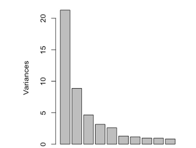
As seen above, the drop in variance after the third principal component is very low, therefore the first three principal components account for the maximum variance in our data (close to 70%). Since the first two principal components consist of the maximum variation in our data, we can analyse their biplots showing their scores and loadings to find any patterns in our data:

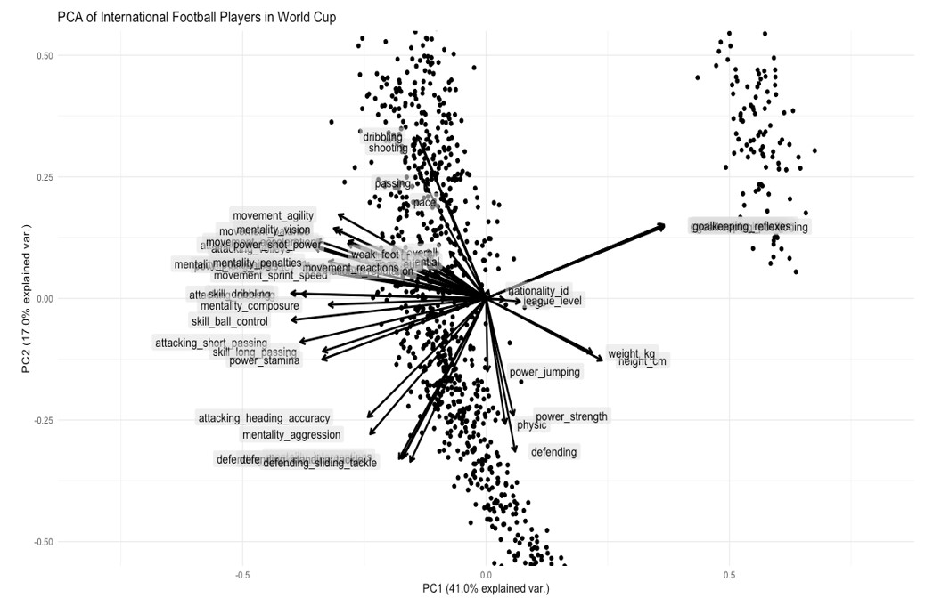
Analysis of Biplot of our PCA

The first principal component shows an interesting contrast. The player with the bigger height and weight will score high on goalkeeping skills. If we increase these attributes, other ones including skill, movement, power, and mentality, will be on the decrease i.e. skills that defenders, midfielders and strikers may have. All the players on right thus must be goalkeepers of their respective teams.

The second principal component shows a contrast between players who score high on skill attributes of a striker such as pace, dribbling, shooting, finishing, agility, speed, reaction, balance etc., and more can be seen on the diagram, but they score lower on attributes that a defender would typically show such as weight, height, long passing etc. This looks like a contrast between strikers and defenders/midfielders. It’s interesting to see that most successful strikers in the game have these kinds of skills. Furthermore, it looks like most modern strikers from many different countries have not only less weight, height and good attacking skills to qualify as a striker but also are paid more wages and are valued more than other positions in the game. We can verify if these skills do translate to a higher value by using a correlation heatmap:

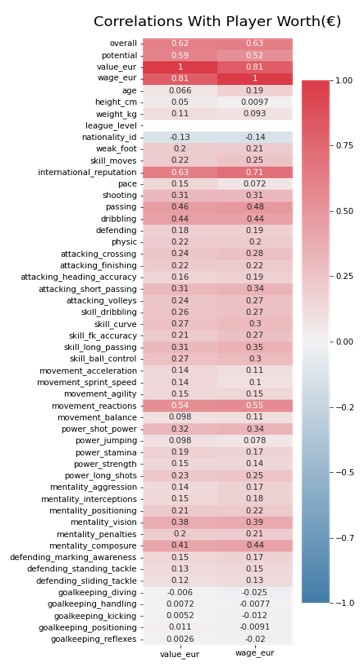
The heatmap above shows that those players with the attributes of a striker are valued more than other positions, as the skills for this position are highly correlated with wages and overall value (light to dark red). It also looks like international reputation, skills for passing, dribbling, reaction and composure are the biggest indicators in descending order of importance of a player’s net worth in the team.

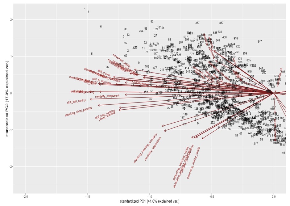
Therefore if we zoom to the left of our biplot, we can say that players at the top are the best strikers in the game and those at the bottom are the best defenders, while the border between these two categories can be thought of as consisting of players who are the best midfielders, which will become clearer when making clusters of our data. Some of the most popular strikers of the game actually do feature in our biplot labelled with their id number in our data frame, such as Messi (1), Neymar (4), Ronaldo (3), Mbappe (6) etc. Some football fans might be displeased as to why Messi is positioned higher than Ronaldo in our analysis, well, numbers do not lie, and having looked it up, it seems like Messi does have more Ballon d’Ors than Ronaldo. The properties that make up a perfect striker are all aligned highly towards Messi, who is at the top left on our biplot.

K-means Clustering

Now that we have a rough idea of how our data has been divided into roughly three categories, we can actually verify if three clusters can be formed from this data or if we are bluffing based on the results from our PCA. The K-means clustering algorithm congregates data into “K” clusters. The challenge we have at our disposal now is finding out the value of K. We will use the silhouette method to find this out. This method measures the average silhouette width for each value of K, a higher value of which indicates good quality of clustering i.e. how well a data point fits within a cluster. We get the following result for our data:

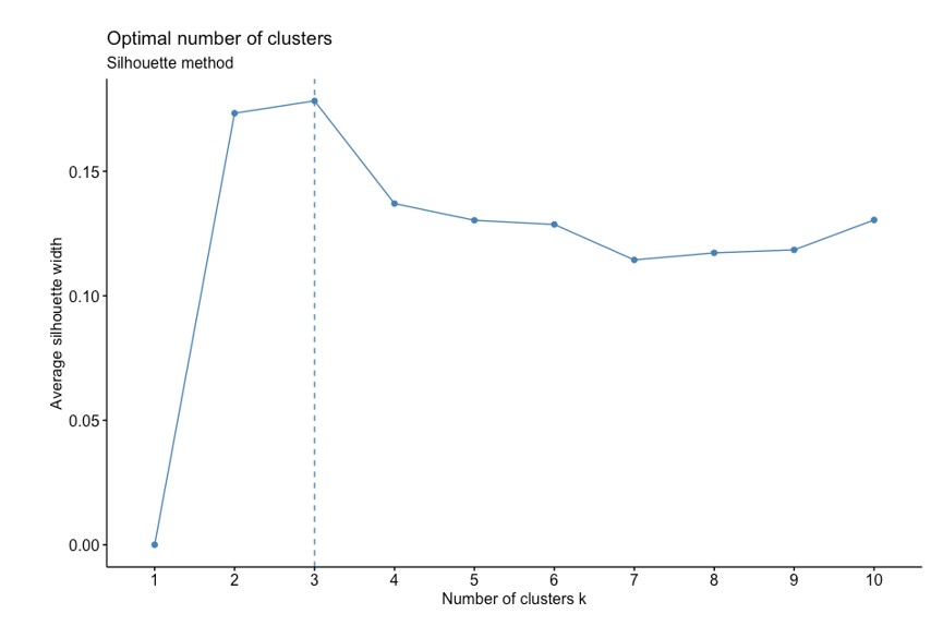
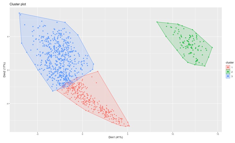
The highest value for average silhouette width before it goes down is 3, so we have now confirmed that the optimal number of clusters for our data should be 3. We get the following clusters plotted on our first two principal components:

Insights from K-means Clustering

Just as we suspected, these 3 clusters are representing the positions in a football match, the goalkeepers are in green, as concluded from our first principal component. As for other clusters, they look like a mixed bag, but generally, strikers are in blue as concluded from our second principal component, those at the top of the graph have the best skills, which make up for a striker, and similarly, defenders/midfielders are in red. The red and blue clusters have a lot of overlap in the middle, so we cannot cluster a certain player in exactly the same place all the time. This forms the border of our cluster, where we can find the best midfielders.

How Has This Analysis Helped us?

At first, unsupervised machine learning has helped us (well, me!) find patterns in our data and what skills make up the best player on the pitch. With so many data points, we first reduced the dimensions of our data and successfully found clusters of players and what makes them unique, then we reverse-engineered through domain knowledge what these clusters could represent.

Suppose we have a player whose attributes we know, but we do not know what category or cluster that player belongs to, i.e. attackers, goalkeepers, defenders or midfielders. We can therefore use machine learning with this data to assign the unknown player a cluster where he will most likely fit in his national team. This just shows how powerful machine learning can be, to not only find insights in our data on which we have no prior domain knowledge but also to then use these results to classify future occurrences.

The Big Question, Who Has the Strongest Overall Team?

This is a tough question to answer, but we can get a rough idea of who has the strongest team based on the overall skill level from the data. The column ‘overall’ in the data frame gives us an average overall score for a player based on taking the average of their average skill attributes. This score looks like a normally distributed curve, as shown below:

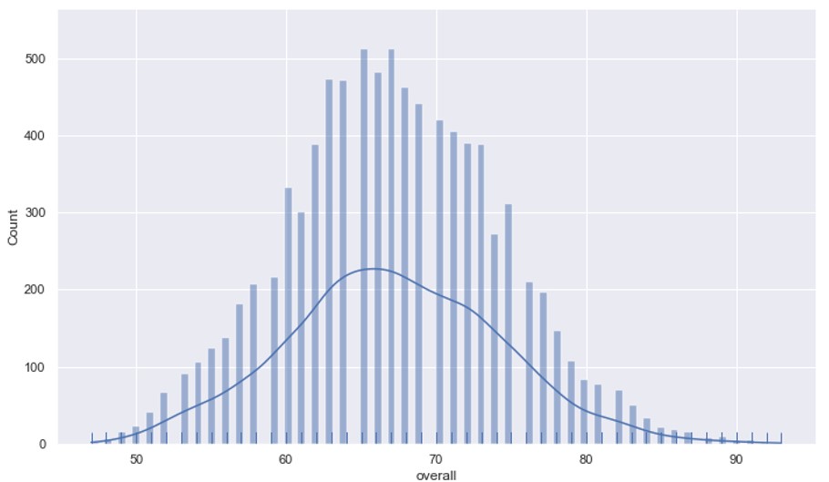
This means players who are the best in the world (overall value closer to 90) in their position within their team are very few (right end of the bell curve) and the same can be said about players who are not so good skill wise (left end of the bell curve). Most players fall in the middle. Therefore, if we aggregate this overall score by the countries participating in the world cup and include league players of all levels within their respective countries, we can rank countries by the average overall score and see which country has the most skilful players (as shown below).

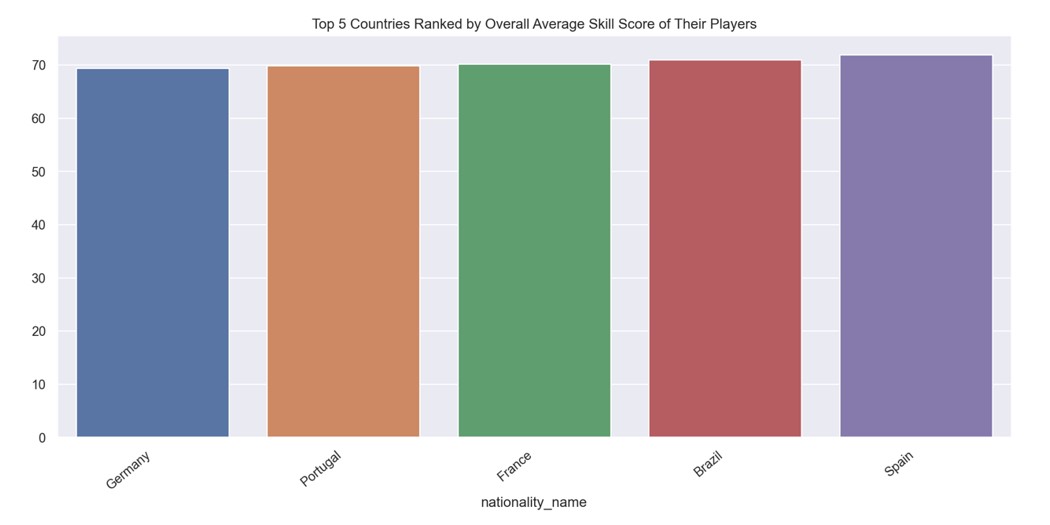
The top 5 teams are extremely close when you average out the skill score of their players, with Spain predicted to have the best chance of winning since they have the most talent skill-wise. However, since the margins between the teams are so small, we cannot statistically determine who has the best chance of winning just based on this feature. Nevertheless, the data indicates that these teams are expected to perform the best in the tournament, with Spain narrowly coming out on top. Our biplots also confirm that the best strikers, defenders, goalkeepers, and midfielders are mostly from these five countries, as evidenced by their high PCA score values.

For more information, get in touch with our specialists to find out more about our Machine Learning services for OCI and Azure. or book a meeting...